The Geometry of Prediction

Disclaimer: These are formal notes based on lecture slides from the Computer Vision course I am currently enrolled in as of March 2026. Permission to share this material was obtained before publishing this article.

In-text hyperlinks throughout this article serve as contextual and prerequisite learning resources. They are included for readers to explore underlying concepts but are not part of the formal reference list, as they were not directly used in the derivation of the material presented.

Introduction

In the previous article on the shift to convolutional neural networks (CNNs) in computer vision tasks, practitioners have classified manual feature engineering as relatively suboptimal compared to the automated learning of hierarchical representations. When we move from purely raw pixel data to semantic class scores in computer vision tasks, both computational and geometric aspects need to be accounted for.

Since classification methods in machine learning have traditionally required image feature classes to inhibit properties of linear separability, this creates a unique issue. These features manifest as high-dimensional manifolds. This means that practitioners are burdened with the task of transforming these features from a high-dimensional space into one in which a hyperplane allows linear separation of classes for classification.

Thus, CNNs and their use in computer vision require a dissection of the linear transformation mathematics that serve as their foundational logic.

We will focus specifically on forward propagation.

This article will highlight the sequence of linear transformations and non-linear activations that enable this mapping from raw input data to final predictions.

Linear Basis of Classification

We will use the CIFAR-10 dataset as an example for our mathematical analysis, a dataset commonly used in machine learning and computer vision.

In deep architectures, such as neural networks, the fundamental building block is the linear classifier. This is where the transition from raw image data to a discrete score space in an arbitrary plane occurs.

We define the scoring function as

$$f(x; W, b) = Wx + b$$

Where:

• $x$ — the input vector. In our example, the standard CIFAR-10 image is a $3072 \times 1$ column vector, derived from the $32 \times 32$ pixel grid across the three color channels Red, Green, and Blue ($32 \times 32 \times 3 = 3072$).
• $W$ — the weight matrix of size $10 \times 3072$. Each row in the matrix serves as a learned high-dimensional template for one of the $10$ classes.
• $b$ — the bias vector ($10 \times 1$), providing a data-independent offset for each class score.

The matrix multiplication $Wx$ computes the inner product between the input image and the learned class templates. In this sense, a linear classifier treats each class as a fixed "template" and scores how well the input matches it. Each row of $W$ can be reshaped and visualized as a kind of "prototype" image for the class it represents.

However, this approach is fundamentally limited. This is due to the stacking of linear layers. No matter how many are stacked, they collapse into a single linear transformation.

As a result, the model can only learn simple, linear decision boundaries and cannot capture the complex, hierarchical patterns — such as shapes and textures — present in real-world images.

For example:

• We "stretch" the input pixels into a single column vector.
• In our abstract example with $4$ pixels and $3$ classes (cat, dog, ship), we then multiply a $3 \times 4$ weight matrix by the pixel column and add a bias term:

$$s \;=\; \begin{pmatrix} w_{11} & w_{12} & w_{13} & w_{14} \\ w_{21} & w_{22} & w_{23} & w_{24} \\ w_{31} & w_{32} & w_{33} & w_{34} \end{pmatrix} \begin{pmatrix} x_1 \\ x_2 \\ x_3 \\ x_4 \end{pmatrix} + \begin{pmatrix} b_1 \\ b_2 \\ b_3 \end{pmatrix}$$

• A composition of multiple linear layers then collapses into a single linear transformation:

$$f_2\!\left(f_1(x)\right) \;=\; W_2\!\left(W_1 x + b_1\right) + b_2 \;=\; \underbrace{(W_2 W_1)}_{W'} x + \underbrace{(W_2 b_1 + b_2)}_{b'} \;=\; W'x + b'$$

This is not robust enough for us. Because linear layers alone represent only simple transformations, we need non-linear activation functions to make the model more expressive and prevent it from collapsing into a single linear operation.

Nonlinearity and Activation Manifolds

To break linearity, we use activation functions, briefly mentioned in the article on the road to CNNs. These functions allow the network to approximate any continuous function. This means that it allows the arbitrary feature spaces to be warped and shifted, creating complex manifolds that can separate data that was not initially separable in its raw form.

Here is a list of some functions that transform pre-activation signals and introduce non-linearity:

Sigmoid

This function takes in a raw score value and "squeezes" it into an "S" curve on the graph that is strictly between the values $0$ and $1$.

$$\sigma(z) \;=\; \frac{1}{1 + e^{-z}}$$

This is useful for converting raw scores obtained from the scoring function into probabilities in a binary classification setting (i.e., deciding between two classes — one or the other), otherwise known as binary logistic regression. An output closer to $1$ indicates confidence in one class, while an output closer to $0$ indicates confidence in the other.

Hyperbolic Tangent

Similarly to the Sigmoid function, the Hyperbolic Tangent ($\tanh$) also creates an "S" curve on the graph.

$$\tanh(z) \;=\; \frac{e^z - e^{-z}}{e^z + e^{-z}}$$

The difference, however, is that its outputs are stretched to fall between $-1$ and $1$. This maps values to a range centered on zero, which helps balance the neural network's weights better than the aforementioned Sigmoid function. Thus, it helps lead to faster and more efficient training convergence.

Softmax

Instead of a singular score value, like the Sigmoid function, this function takes in a vector of raw score values.

$$\mathrm{softmax}(z)_i \;=\; \frac{e^{z_i}}{\sum_{j=1}^{K} e^{z_j}}$$

This also "squeezes" the scores into a probability distribution, where each value lies between $0$ and $1$. This is useful for converting raw scores into probabilities in a multi-class classification setting (i.e., deciding among more than two classes), otherwise known as multiclass logistic regression. An output closer to $1$ for a given class indicates higher confidence in that class relative to the others, while lower values indicate less confidence.

Rectified Linear Unit (ReLU)

This is a function that leaves positive values unchanged while turning all negative values to $0$.

$$\mathrm{ReLU}(z) \;=\; \max(0, z)$$

This effectively disregards negative inputs, thereby creating sparsity (when only some neurons in a neural network are active at a given time). As a result, the function is computationally fast and efficient.

In the previous article, we mentioned that this simplifies backpropagation and speeds up learning while also addressing the vanishing gradient problem, where gradients shrink exponentially and prevent early layers from learning. Since older activation functions like Sigmoid and Tanh are prone to this issue, ReLU is a more effective choice.

However, this strict non-negativity can lead to a problem known as the "dying neuron" problem, in which neurons in a neural network that consistently receive negative inputs stop learning entirely.

Leaky ReLU

To fix the "dying neuron" problem, instead of turning negative inputs directly to zero, this function modifies the original ReLU function by allowing some "leaking," meaning it permits a small, non-zero output for negative input values rather than completely collapsing them to zero during the backpropagation process.

$$\mathrm{LeakyReLU}(z) \;=\; \begin{cases} z & \text{if } z > 0 \\ \alpha z & \text{if } z \leq 0 \end{cases} \qquad \text{with small } \alpha > 0$$

Maxout

This function takes the maximum value from $n$ linear functions. By piecing together multiple lines (each representing a linear function in the $\max$ operation), it can learn to approximate the shape of any convex function (ReLU or a quadratic curve).

$$\mathrm{Maxout}(x) \;=\; \max_{i \in \{1, \ldots, n\}} \left( w_i^\top x + b_i \right)$$

Because of this flexibility, networks using it are considered universal approximators.

Exponential Linear Unit (ELU)

This function is similar to ReLU in that, for positive inputs, ELU behaves like a straight diagonal line. However, it handles negative inputs differently.

$$\mathrm{ELU}(z) \;=\; \begin{cases} z & \text{if } z > 0 \\ \alpha\!\left(e^{z} - 1\right) & \text{if } z \leq 0 \end{cases}$$

This is because instead of cutting them off, it maps them to a smooth curve that approaches a minimized negative limit. This smooth transition helps stabilize gradient optimization, speeding up the learning process.

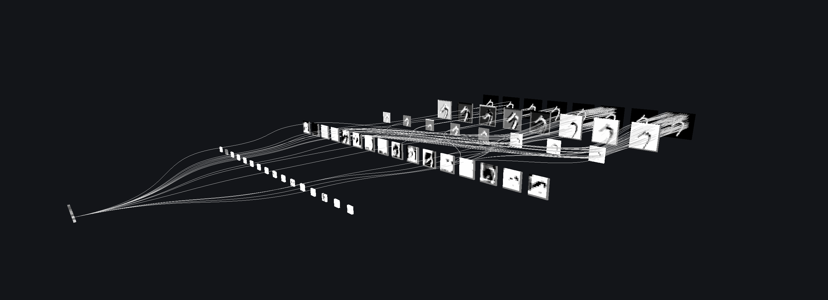
Hierarchical Feature Extraction via Forward Propagation

In the section from the previous article, Pixels to Objects, the first layers of the neural network detect local edges, the second layers combine them into corners or parts, and higher layers build abstract features that recognize entire objects. This logic is synthesized into the following graph, assuming a 3-layer neural network structure:

Let us build a formula based on these assumptions.

Input Projection (Linear Combination)

We take the input features and compute the pre-activation weighted sum for each hidden unit. This yields our linear scoring function value:

$$z_j \;=\; \sum_{i=1}^{D} w_{ji} \, x_i + b_j \qquad \text{or, in matrix form,} \qquad z \;=\; Wx + b$$

This step projects the raw input data into a new space, where each hidden unit captures a different combination of input features. $D$ is designated as the input's dimensionality.

Non-linear Activation Function

With the weighted sum of each hidden unit, we then pass this value through a non-linear activation function (could be any of the aforementioned functions mentioned in the previous section).

$$h_j \;=\; \phi(z_j) \qquad \text{or} \qquad h \;=\; \phi(z)$$

This is what gives the neural network the ability to transcend beyond linear relationships and capture more complex patterns in the data.

Output Aggregation

The activated hidden units are then combined to produce an output via weighted summing:

$$s_k \;=\; \sum_{j=1}^{M} v_{kj} \, h_j + c_k \qquad \text{or, in matrix form,} \qquad s \;=\; V h + c$$

In this step, the neural network aggregates all of the information from the hidden units to form a separate output score for each output class. $M$, in this case, denotes the number of hidden units.

Prediction

With our output scores for each class, we apply an output function that converts the scores into interpretable probabilities:

$$\hat{y} \;=\; g(s)$$

Some output function options include:

• Sigmoid for $2$ classes.
• Softmax for multiple classes.

In essence:

• The first transformation extracts basic features from the input.
• Then non-linearity allows these features to interact in complex ways.
• Finally, the last layer combines them to make a prediction.

Thus:

$$\hat{y} \;=\; g\!\left( V \, \phi(Wx + b) + c \right)$$

Computer vision has shifted from manual feature engineering to models that learn hierarchical representations automatically.

Tl;dr

• Raw pixel data must be transformed into a space where classes can be linearly separated, but real-world image features form complex, high-dimensional manifolds.
• A linear classifier performs template matching using $Wx + b$, scoring how well an input aligns with learned class prototypes.
• However, stacking linear layers does not increase model power — they collapse into a single linear transformation.
• This limits the model to simple decision boundaries, making it incapable of capturing complex visual patterns.
• To overcome this, neural networks use non-linear activation functions, which allow them to:
  • Warp feature spaces
  • Model complex relationships
  • Separate non-linearly separable data
• Common activation functions include:
  • Sigmoid → binary probabilities
  • Tanh → zero-centered outputs
  • Softmax → multi-class probability distribution
  • ReLU → efficient, sparse activation (but can "die")
  • Leaky ReLU / ELU / Maxout → improvements addressing ReLU limitations
• Forward propagation in a neural network follows a structured pipeline:
  • Input projection → weighted sums (linear scoring)
  • Non-linearity → transforms features
  • Output aggregation → combines hidden representations
  • Prediction → converts scores to probabilities

This entire process compresses the intuition of:

edges → parts → objects

All into a single mathematical expression describing the network's behavior:

$$\hat{y} \;=\; g\!\left( V \, \phi(Wx + b) + c \right)$$

References

1. Das, S. Deep Learning — Convolutional Neural Networks (Lectures 9). ITCS-4152 / ITCS-5010 Computer Vision course lecture slides.
2. Jain, R. Maxout — Learning Activation Function. Medium article, Feb. 6, 2020.
3. GeeksforGeeks. Tanh Activation in Neural Network. GeeksforGeeks article, Last Updated: Feb. 14, 2025.
4. GeeksforGeeks. Softmax Activation Function in Neural Networks. GeeksforGeeks article, Last Updated: Nov. 17, 2025.
5. GeeksforGeeks. Sigmoid Function. GeeksforGeeks article, Last Updated: Jul. 23, 2025.
6. GeeksforGeeks. ReLU Activation Function in Deep Learning. GeeksforGeeks article, Last Updated: Jul. 23, 2025.
7. GeeksforGeeks. Leaky ReLU Activation Function in Deep Learning. GeeksforGeeks article, Last Updated: Jul. 12, 2025.
8. GeeksforGeeks. ELU Activation Function in Neural Network. GeeksforGeeks article, Last Updated: Jul. 23, 2025.

Further Reading

• The Road to Convolutional Neural Networks