What Happens Below a Machine Learning Framework?
Tensors, autodiff, and Compiler Representations on a High-level
SEP 4 · 2026 · 14 MIN READ
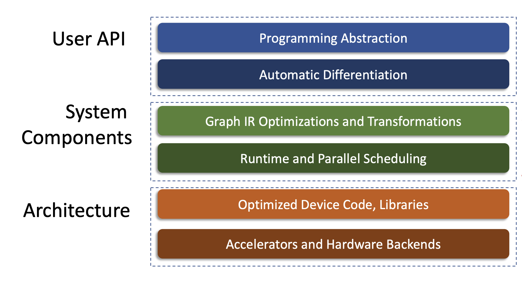
Prerequisite knowledge is required to understand every part of this article in full. Fret not, as I will do my best to provide in-text links and citations for much of the information within this article, including the prerequisite knowledge, which some won’t formally be in the references section. The in-text citations may be broad or vague regarding the definition of the hyperlinked word, but are connected to the context clues within this article when researched. All notation shown is original unless cited otherwise.
If you have ever navigated and implemented the process of building, training, and subsequent deployment of a deep learning model or neural network, one of the most accessible and common ways is to utilize what are called general libraries, which are programming libraries that one can import into their codebase that provide pre-made and ready-for-use code.1 Examples of ML frameworks include PyTorch, TensorFlow, and JAX. These frameworks provide a common toolset for the user and programmer to express mathematical intention, since the AI tasks, algorithms, and models are pre-built, without having to manage the actual machinery needed to do the math on the hardware directly.2
To demonstrate these abstractions, we will construct a simple neural network’s forward propagation and backpropagation mechanisms:
If we want to take an input of data and a set of learned knobs and configurations, i.e., weights that control how the input is transformed, we can then yield the neural network’s prediction, .1 This is denoted as
For matrix multiplication to occur, the dimensions of two matrices must align. From linear algebra fundamentals, this means the number of columns in the first matrix must match the number of rows in the second.
So, with the data and the weight possessing the attribute of being an -sized matrix and a -sized matrix, respectively, this expression can be extended to
Thus, if we fully expand the notation of these matrices out, the multiplication actually looks like
More accurately, in ML frameworks and fundamentals, the arbitrarily sized data matrix , weight matrix , and output/prediction matrix are better understood as tensors (which serves as an important definition and semantic backbone later on, as you will see). The number of dimensions in a tensor is called the rank.
In our previous matrices , , and , since there were two dimensions — , and — per matrix, these matrices would be categorized as rank-2 tensors.
And, since tensors can have arbitrarily sized dimensions, we can use , , and to denote the individual tensor ranks for , , and , respectively, and , , and to denote some assigned value/size of each dimension, also respectively. Therefore,
In Python-based ML frameworks, this is commonly written using the @ operator, which signifies matrix multiplication operations and tensor contractions/manipulations.
y = x @ WThis is our linear transformation used in this simplified forward propagation mechanism.3
Now we have our prediction value from forward propagation, , at our disposal. However, we want our neural network to be able to learn things, so ideally, we would want to compare the value of the prediction to the correct answer of whatever the neural network is trying to learn, which we will instantiate as . This very comparison is called a loss function, which can be denoted as
Fundamentally, you can think of backpropagation as moving backwards from a forward propagation. We are trying to figure out which learned knobs contributed to how off the prediction was. This means we want to figure out how wrong the neural network’s prediction was and subsequently which learned knobs caused the network to be wrong and by how much.
So, we want to know how sensitive the loss function result is to changes in the weight matrix by taking the partial derivative of with respect to :
And, if , this can be visualized as a rank-2 tensor (matrix) collection of partial derivatives, denoted as what can be referred to as the gradient of the loss4:
One way is to denote a single entry of the loss 's local sensitivity to one particular weight , inside the gradient, such that
where denotes the row number of the matrix and denotes the column number. This makes a scalar value; a rank-0 tensor.
To articulate multiple entries within the gradient that follows an assumption of , then
A complete gradient containing the derivatives with respect to (w.r.t.) every component of is formalized in notation in a way that distinguishes generalizability regardless of the rank of , given the loss is scalar-valued:
Thus, in this paradigm, there exists an equivalence, such that
Therefore,
Remember that the loss is not only yielded from changes in the weight matrix . In order for the prediction , it requires (forward propagation), and the prediction is important for computing . If you want to understand how influences , the dependency path backwards could be thought of as
Following the line of dependencies — depends on which depends on — we can invoke the chain rule from calculus, such that
Where indexes the rows of , and indexes the columns of .
To put it all together, if we take our forward propagation mechanism, , and we want to back-propagate/find the gradient of the loss w.r.t. , we will take the transpose of so that we maintain the matrix dimensions and align it for matrix multiplication, such that
So when
then
And if we wanted to find the gradient of the loss w.r.t. data input , then it works the same way:
In PyTorch, this entire backward mechanism is triggered using a very simple line of code:
loss.backward()In TensorFlow,
tf.GradientTapeAnd in JAX,
jax.gradThis is our backpropagation mechanism.
Already, off the bat, we can see how y = x @ W and loss.backward() are simple lines of code that act, in and of themselves, as an abstraction of the mathematics in formal articulation. For these lines of code, sprawling software-to-hardware relationships with foundational robustness must exist; y = x @ W can perform a forward pass with ease, and loss.backward() can elegantly trigger a series of backward-chained derivatives in a neural network. This is where the even deeper abstractions reside.
Underneath y = x @ W
PyTorch stores information like the data type, device, and layout when defining a tensor.3 Intuitively, the tensor’s shape tells the framework the dimensions of the data, and the layout and related metadata signal how that tensor is arranged and accessed in memory.
This is important when we analyze the perspective in which a piece of hardware takes upon a tensor’s presence: a matrix and a matrix have their values stored ultimately within a hardware system’s memory locations. This means that before an operation like @ can be validated and executed, a computer system must know whether the tensors are on a CPU, on an accelerator card, or in some other memory space. Within these constraints, the system must know a tensor’s dimensionality compatibility, memory layout, and whether it is suitable for the operation requested.
So, within the software-to-hardware dynamic, when y = x @ W is invoked, a framework must resolve what kind of tensor operation is being requested and choose an implementation based on it; a process that can be broadly understood as an operation dispatch. Depending on different tensor attributes, this operation dispatch can look different across the board.
We can get even lower than this; this was merely the software side of the hardware boundary here. There exists even more concreteness within the y = x @ W expression. As mentioned earlier, the matrix multiplication operation needs memory allocation, layout conversion, scheduling the processes and tasks around the operation, and hardware-specific kernels. As mentioned earlier, a great example is Tenstorrent’s open software stack, which separates the higher-level compiler and operation interfaces from the low-level programming and metal through the TT-Metalium repository.2, 4
As a wrap-up, not every ML framework adheres to the same philosophy, you could say, on how it handles something like Python code all the way down to hardware execution. For a system to turn y = x @ W into a concrete plan, it must understand the tensors and validate the operation invoked upon them. Then it chooses an implementation, manages the memory space, and then it finally performs the real work on the metal.
Underneath loss.backward()
The result of y = x @ W is a prediction value . Within a neural network, and its structure as previously stated, a comparison between the prediction and the correct answer is made via the loss , yielded from the loss function . The process of backpropagation is to determine how changes in the learned weight values affect the loss, which is crucial for how a neural network actually learns; it tries to understand how much the internal learned knobs of the model contributed to the error of the output, and compute the gradients needed for the optimization step needed to update the weights .
Recall that when loss.backward() is invoked, the abstraction is actually the backwards computation of partial derivatives through the chain rule from calculus. ML frameworks must know which intermediate values the operations depend on, and how and in what order gradient information should be organized and subsequently propagated backwards through the network. This is where the concept of automatic differentiation, or autodiff, comes from.
Take micrograd as an example. Micrograd is a small, scalar-valued, reverse automatic differentiation engine (autograd) developed by Andrej Karpathy as an educational implementation of what lies underneath an ML framework during backpropagation. A dynamically constructed directed acyclic graph (DAG) is instantiated, which helps the engine remember the operations that produced the values from forward propagation, which previous values existed/depended on, and what local backward rule should be applied. In simpler terms, this all leaves a trail/record of how the loss value came to be.
This record-keeping structure can, at times, demonstrate that one value within this chain can affect the final loss value through multiple computational paths. The same weight can be used in multiple later operations, which means several downstream pieces can be affected when it comes to contributing toward that said weight’s final gradient. Before gradients are propagated backwards, the system has to traverse the DAG in an order that respects how each value was used. In Karpathy’s micrograd, it builds this topological ordering of a DAG before it applies the backward chain rules.
If we scale this ML framework infrastructure — to the size of PyTorch — the autograd mechanics follow the same broad idea. As tensor operations execute, PyTorch will construct this graph of backward Function objects. These intermediate values are saved and called upon when needed for future derivative calculations. Then, upon calling loss.backward(), autograd uses these operation history records to compute gradients. Ultimately, the goal is to preserve enough information during the forward pass so that the backwards pass can later apply the chain rule correctly.
In this sense, you could say that loss.backward() sits just one layer above the execution machinery that was discussed earlier. If you think of autograd as deciding what gradient work must happen, and the ML framework deciding how that work will run, on an accelerator-oriented stack, one could imagine it also eventually involving intimate tinkering with runtime execution, memory allocation, device-specific kernels, and the movement of tensor data through memory, just like forward pass operations require as well! 4, 2
Compiler Representations - High Level
Fundamentally, operation dispatch and execution models are related, but are separate decisions; operation dispatch selects an implementation for an operation, while execution models determine whether operations are issued immediately or captured into a larger representation.
Frameworks like PyTorch and TensorFlow, along with their compiler/runtime stacks, vary widely in how they handle the same line of y = x @ W code due to operation dispatch/implementation choices. Broadly, this means that the way PyTorch, TensorFlow, JAX, tinygrad, some TVM or MLIR-based systems, or hardware-specific stacks like Tenstorrent’s systems handle code, regarding operations and their subsequent implementations, is, unsurprisingly, different from one another.
For example, two different handling styles — eager execution systems and graph/compiler-oriented systems — represent two different execution styles:
-
In an eager execution system, an operation is issued when the program reaches it. This style is useful, intuitive, makes the program feel more direct, and can be debugged relatively easily. Simply: write an operation, run the operation, receive the result.
- PyTorch is an example of a framework that uses this style by default; however, it also has graph/compiler-oriented systems as an option.
-
In graph/compiler-oriented systems, an operation may be captured into a larger representation before it is executed. This is because some systems retain a larger region of computation before an operation executes. This allows scheduling and lowering high-level tensor operations into lower-level representations and target-specific programs.
-
tinygrad is an example of a framework: they show documentation and an example of a system that moves from an abstracted Tensor API/frontend into UOps, scheduling, lowering, compilation, and runtime execution.
-
As an extension, there are broader compiler examples as well regarding retaining computation in intermediate representations (IR), which makes operations easier to analyze, transform, and subsequently optimize before it reaches the hardware.5, 6
-
In the exploratory pursuit of software-to-hardware dynamics, there exists a distinction between the gradient computation graphs and compiler IRs. You could think of an autograd graph as asking “how was this loss produced, and how should the gradient be computed?” The compiler IR would ask, “Well, how would this computation be represented, conditioned to the fact that it needs to be optimized and subsequently mapped into a target execution system?”
These roles are distinct, but they are not mutually exclusive: some systems perform automatic differentiation as a transformation over an intermediate representation, and computations produced by autodiff may later be captured and compiled.
As we descend deeper into the abstractions, and into the compiler representation side of things — i.e., intermediate representations — it is important to note that reverse-mode autodiff does not require the representation known as Static Single Assignment (SSA). In many compiler tasks, SSA can be useful; however, it is not a prerequisite for autodiff specifically. Micrograd is an example of this, since its reverse-mode autodiff is actually implemented via ordinary Python objects connected through the dynamic DAG rather than this compiler IR approach.7
Conclusion
To keep this article epistemically grounded, avoid scope creep, and not get too ahead of ourselves with the series of future articles succeeding this one — foundations for a much larger project — I want to conclude this piece. Already, our rudimentary instantiation of a basic forward and backward pass reveals the hidden layers of tensors, operation dispatch, compiler stuff, and autograd. Not every ML framework implements forward propagation or backpropagation the same way, with the same internal machinery.
References
Main References
- D. Zax, “Top Machine Learning Libraries,” IBM Think. [Online]. Available: https://www.ibm.com/think/topics/machine-learning-libraries. Accessed: Sep. 2, 2026.
- Tenstorrent, “Software Overview,” Tenstorrent Documentation. [Online]. Available: https://docs.tenstorrent.com/software/index.html. Accessed: Sep. 2, 2026.
- PyTorch, “Tensor Attributes,” PyTorch Documentation, ver. 2.13. [Online]. Available: https://docs.pytorch.org/docs/2.13/tensor_attributes.html. Accessed: Sep. 2, 2026.
- Tenstorrent, “TT-Metalium Documentation,” Tenstorrent Documentation. [Online]. Available: https://docs.tenstorrent.com/tt-metal/latest/tt-metalium/index.html. Accessed: Sep. 2, 2026.
- C. Lattner, M. Amini, U. Bondhugula, A. Cohen, A. Davis, J. Pienaar, R. Riddle, T. Shpeisman, N. Vasilache, and O. Zinenko, “MLIR: Scaling compiler infrastructure for domain specific computation,” in 2021 IEEE/ACM International Symposium on Code Generation and Optimization (CGO), 2021, pp. 2–14, doi: 10.1109/CGO51591.2021.9370308.
- T. Chen, T. Moreau, Z. Jiang, L. Zheng, E. Yan, H. Shen, M. Cowan, L. Wang, Y. Hu, L. Ceze, C. Guestrin, and A. Krishnamurthy, “TVM: An automated end-to-end optimizing compiler for deep learning,” in 13th USENIX Symposium on Operating Systems Design and Implementation (OSDI 18), Carlsbad, CA, USA, 2018, pp. 578–594. [Online]. Available: https://www.usenix.org/system/files/osdi18-chen.pdf.
- A. Karpathy, “micrograd: A tiny scalar-valued autograd engine and a neural net library on top of it with PyTorch-like API,” GitHub. [Online]. Available: https://github.com/karpathy/micrograd. Accessed: Sep. 2, 2026.
Additional Sources
- T. Chen, “ML Frameworks and Abstractions,” 15-884: Machine Learning Systems, Carnegie Mellon University, Spring 2021. [Online]. Available: https://catalyst.cs.cmu.edu/15-884-mlsys-sp21/slides/1-MLSys-MLFrameworkAbstraction.pdf. Accessed: Sep. 7, 2026.
In-Text Links
- Deep learning — introductory definition
- Neural network — beginner’s guide
- General libraries — machine-learning libraries
- PyTorch documentation
- TensorFlow learning resources
- JAX documentation
- Forward propagation
- Backpropagation
- Compatible matrices — dimension requirements
- Tensors
- Tensor rank
- Loss function
- Gradient of the loss
- Chain rule from calculus
- Matrix transpose
- Metadata
- Underlying tensor values
- Tensor attributes — data type, device, and layout
- Memory locations
- Central processing unit
- Accelerator cards
- Row-major memory layout
- PyTorch matrix multiplication
- PyTorch operation dispatch
- Memory allocation for kernel developers
- Hardware-specific matrix-multiplication kernel
- TT-Metalium repository
- Gradient information
- Automatic differentiation
- micrograd
- Reverse-mode automatic differentiation
- Andrej Karpathy
- Dynamically constructed directed acyclic graph
- Final loss value
- Final gradient
- Topological ordering of a DAG
- tinygrad developer documentation
- TVM
- MLIR
- Tenstorrent software overview
- Eager execution systems
- Graph/compiler-oriented systems
- JAX computation capture
- tinygrad scheduling
- tinygrad lowering
- tinygrad Tensor API/frontend
- UOps
- tinygrad compilation
- tinygrad runtime execution
- Intermediate representations
- Static Single Assignment
- Bias term
- Tensor contractions
- Activation function